Flexible Jupyter Notebook for Time Series Forecasting that runs on Microsoft Fabric or locally

I recently looked at using Microsoft Fabric to analyze time series data and be able to use machine learning to forecast future data.
I came across this great example that shows how to build a program to forecast time series data that has seasonal cycles. It uses the NYC Property Sales dataset with dates ranging from 2003 to 2015 published by NYC Department of Finance on the NYC Open Data Portal.
My goal was to be able to run the notebook shown both in Fabric and locally on my computer using Pyspark.
Running in Microsoft Fabric
To use Fabric, you can sign up for a free Microsoft Fabric trial.
Once in Fabric, you need to create a new notebook and a lakehouse to store data for the example. For detailed information, see Add a lakehouse to your notebook.
Create the required resources
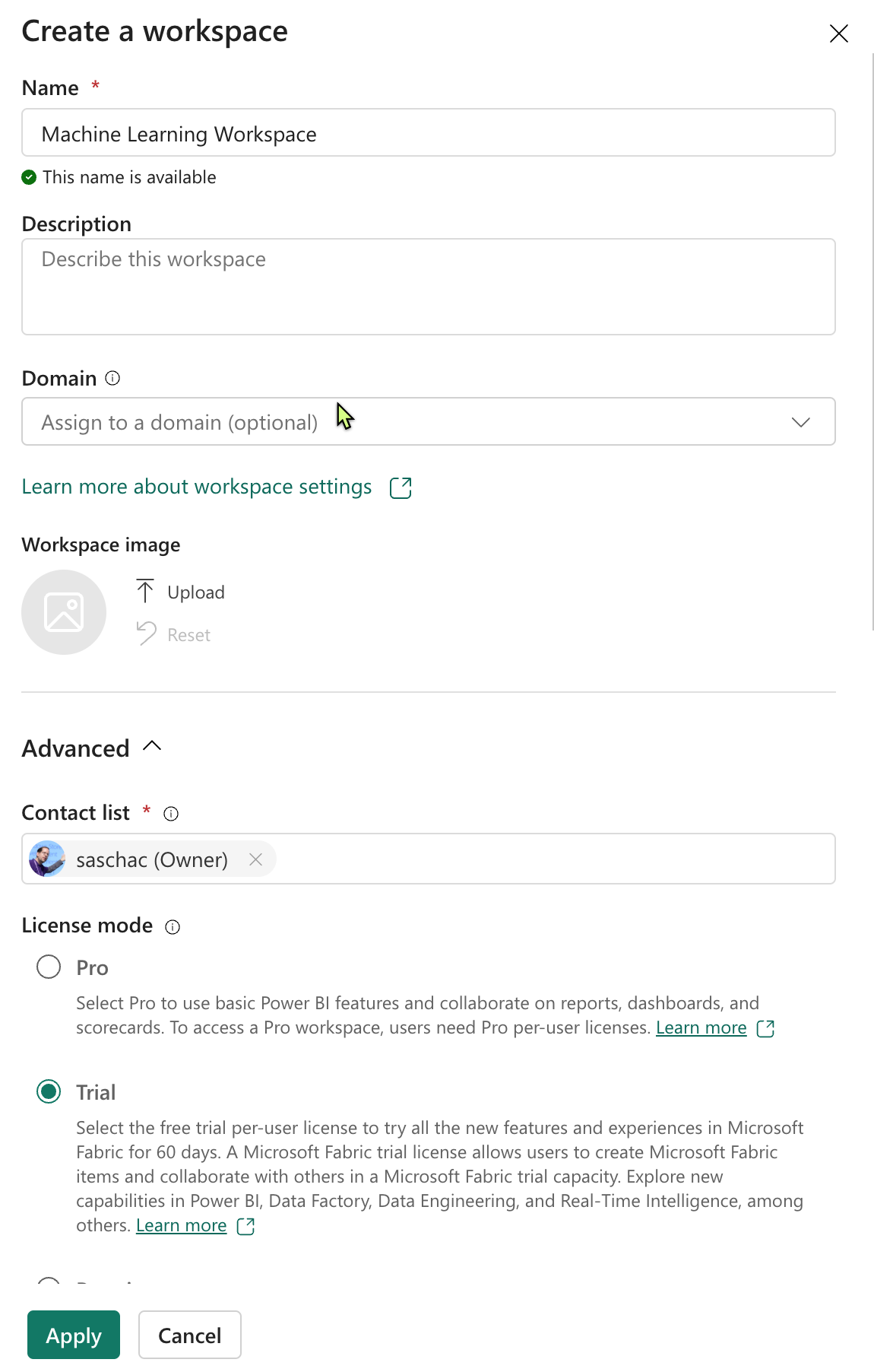
First, create a new Workspace in Fabric.
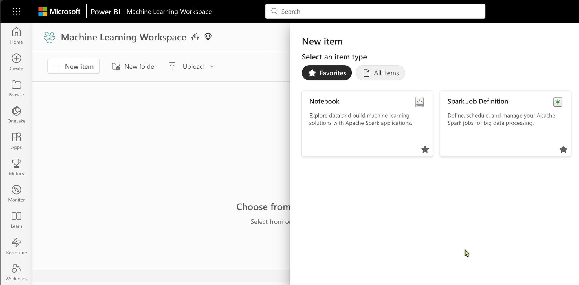
In the new workspace, create a new notebook.
In the notebook, find the Lakehouses...
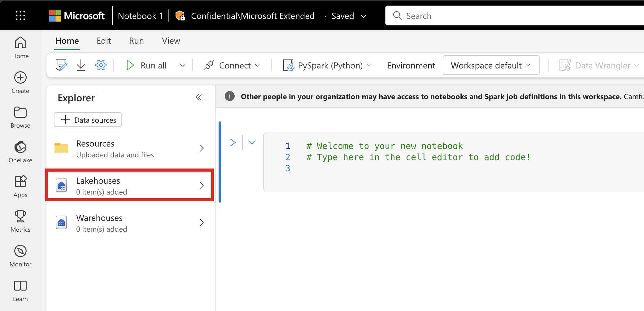
...and create a "New Lakehouse".
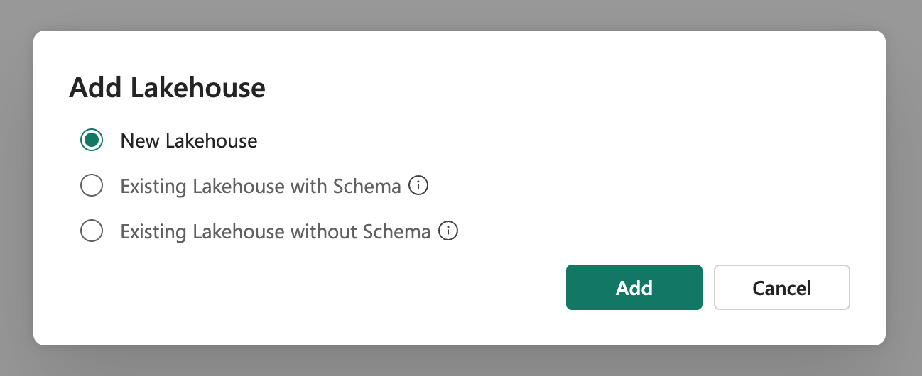
And give it a name.
Now you can start adding the cells to the notebook.
# Time Series Workbook

Configured to run in Microsoft Fabric with attached Lakehouse or locally in VS Code.
Install Libraries if required
When you develop a machine learning model, or you handle ad-hoc data analysis, you may need to quickly install a custom library (for example, prophet in this notebook) for the Apache Spark session.
import os

# Install Prophet if it's missing.
try:
    import prophet
except ImportError:
    %pip install prophet
    import prophet
This helper function is_fabric() will help determine if the notebook is running in Fabric or locally do help figure out if we need to access the lakehouse or the local storage and if we need a Pyspark session.
def is_fabric() -> bool:
    try:
        import synapse.ml.predict
        return True
    except ImportError:
        return False

print(f"Running in Fabric: {is_fabric()}")
Add constants for the paths we will be using.
# Determine base folder based on whether we are running in Fabric or not
BASE_FOLDER = "./data" if not is_fabric() else "/lakehouse/default"

# Setup download folders
URL = "https://synapseaisolutionsa.blob.core.windows.net/public/NYC_Property_Sales_Dataset/"
TAR_FILE_NAME = "nyc_property_sales.tar"
DATA_FOLDER = "Files/NYC_Property_Sales_Dataset"
TAR_FILE_PATH = f"{BASE_FOLDER}/{DATA_FOLDER}/tar/"
CSV_FILE_PATH = f"{BASE_FOLDER}/{DATA_FOLDER}/csv/"

EXPERIMENT_NAME = "aisample-timeseries" # MLflow experiment name
Create a Spark session.
from pyspark.sql import SparkSession
import pandas as pd

def get_spark() -> SparkSession:
    if SparkSession.getActiveSession() is None:
        from delta import configure_spark_with_delta_pip

        builder = (
        SparkSession.builder
            .config("spark.master", "local[*]")
            .config("spark.driver.host", "localhost")
            .config("spark.sql.extensions", "io.delta.sql.DeltaSparkSessionExtension")
            .config("spark.sql.catalog.spark_catalog", "org.apache.spark.sql.delta.catalog.DeltaCatalog")
        )

        local_spark = configure_spark_with_delta_pip(builder).getOrCreate()
        local_spark.catalog.clearCache()
        return local_spark
    return SparkSession.getActiveSession()

spark = get_spark()
Import the Data
The data source consists of 15 .csv files. These files contain property sales records from five boroughs in New York, between 2003 and 2015. For convenience, the nyc_property_sales.tar file holds all of these .csv files, compressing them into one file. A publicly available blob storage hosts this .tar file. We'll download and extract this file.
# Download data
if not os.path.exists(BASE_FOLDER):
    if is_fabric():
    # Add a lakehouse if the notebook has no default lakehouse
    # A new notebook will not link to any lakehouse by default
        raise FileNotFoundError(
            "Default lakehouse not found, please add a lakehouse for the notebook."
        )
    else:
        os.makedirs(BASE_FOLDER, exist_ok=True)
else:
    # Verify whether or not the required files are already in the lakehouse, and if not, download and unzip
    if not os.path.exists(f"{TAR_FILE_PATH}{TAR_FILE_NAME}"):
        os.makedirs(TAR_FILE_PATH, exist_ok=True)
        os.system(f"wget {URL}{TAR_FILE_NAME} -O {TAR_FILE_PATH}{TAR_FILE_NAME}")

    os.makedirs(CSV_FILE_PATH, exist_ok=True)
    os.system(f"tar -zxvf {TAR_FILE_PATH}{TAR_FILE_NAME} -C {CSV_FILE_PATH}")
Set up the MLflow experiment tracking
Start recording the run-time of this notebook and set up the MLflow experiment tracking. To extend the MLflow logging capabilities, autologging automatically captures the values of input parameters and output metrics of a machine learning model during its training. This information is then logged to the workspace, where the MLflow APIs or the corresponding experiment in the workspace can access and visualize it.
# Record the notebook running time
import time
import mlflow

ts = time.time()

# Set up the MLflow experiment
mlflow.set_experiment(EXPERIMENT_NAME)
mlflow.autolog(disable=True)  # Disable MLflow autologging
Read raw date data from the lakehouse and display the DataFrame.
# Read raw data from lakehouse
df = (
    spark.read.format("csv")
    .option("header", "true")
    .load(f"{'' if is_fabric() else BASE_FOLDER+'/'}Files/NYC_Property_Sales_Dataset/csv")
)

display(df)
Exploratory data analysis
Use type conversion and filtering to transform the data into a more suitable format for machine learning. See this link for a description of what is being done in detail.
The data resource tracks property sales on a daily basis, but this approach is too granular for this notebook. Instead, we aggregate the data on a monthly basis.
Aggregate the sale_price, total_units and gross_square_feet values by month. Then, group the data by month, and sum all the values within each group.
Finally, we do a Pyspark to Pandas conversion. Pyspark DataFrames handle large datasets well. However, due to data aggregation, the DataFrame size is smaller. This suggests that you can now use pandas DataFrames.
# Type conversion and filtering
# Import libraries
import pyspark.sql.functions as F

from pyspark.sql.types import IntegerType

df = df.withColumn(
    "sale_price", F.regexp_replace("sale_price", "[$,]", "").cast(IntegerType())
)
df = df.select("*").where(
    'sale_price > 0 and total_units > 0 and gross_square_feet > 0 and building_class_at_time_of_sale like "A%"'
)

# Aggregation on monthly basis
monthly_sale_df = df.select(
    "sale_price",
    "total_units",
    "gross_square_feet",
    F.date_format("sale_date", "yyyy-MM").alias("month"),
)
display(monthly_sale_df)

summary_df = (
    monthly_sale_df.groupBy("month")
    .agg(
        F.sum("sale_price").alias("total_sales"),
        F.sum("total_units").alias("units"),
        F.sum("gross_square_feet").alias("square_feet"),
    )
    .orderBy("month")
)

display(summary_df)

# Pyspark to Pandas conversion
df_pandas = summary_df.toPandas()
display(df_pandas)
Visualization
You can examine the property trade trend of New York City to better understand the data. This leads to insights into potential patterns and seasonality trends. Learn more about Microsoft Fabric data visualization at this resource.
# Visualization

import matplotlib.pyplot as plt
import seaborn as sns
import numpy as np

f, (ax1, ax2) = plt.subplots(2, 1, figsize=(35, 10))
plt.sca(ax1)
plt.xticks(np.arange(0, 15 * 12, step=12))
plt.ticklabel_format(style="plain", axis="y")
sns.lineplot(x="month", y="total_sales", data=df_pandas)
plt.ylabel("Total Sales")
plt.xlabel("Time")
plt.title("Total Property Sales by Month")

plt.sca(ax2)
plt.xticks(np.arange(0, 15 * 12, step=12))
plt.ticklabel_format(style="plain", axis="y")
sns.lineplot(x="month", y="square_feet", data=df_pandas)
plt.ylabel("Total Square Feet")
plt.xlabel("Time")
plt.title("Total Property Square Feet Sold by Month")
plt.show()
Model training and tracking
Model fitting
Prophet input is always a two-column DataFrame. One input column is a time column named ds, and one input column is a value column named y. The time column should have a date, time, or datetime data format (for example, YYYY_MM). The dataset here meets that condition. The value column must be a numerical data format.
For the model fitting, you must only rename the time column to ds and value column to y, and pass the data to Prophet. Read the Prophet Python API documentation for more information.
from prophet import Prophet

# Model Fitting
df_pandas["ds"] = pd.to_datetime(df_pandas["month"])
df_pandas["y"] = df_pandas["total_sales"]

def fit_model(dataframe, seasonality_mode, weekly_seasonality, chpt_prior, mcmc_samples):
    m = Prophet(
        seasonality_mode=seasonality_mode,
        weekly_seasonality=weekly_seasonality,
        changepoint_prior_scale=chpt_prior,
        mcmc_samples=mcmc_samples,
    )
    m.fit(dataframe)
    return m
Cross validation
Prophet has a built-in cross-validation tool. This tool can estimate the forecasting error, and find the model with the best performance.
The cross-validation technique is a valuable tool for evaluating the efficiency of a statistical model. It involves training the model on a subset of the dataset and then testing it on a previously unseen subset. This process helps assess how well the model generalizes to an independent dataset. However, this approach faces a challenge when dealing with time-series data. If the model has already seen data from a specific period, such as January 2005 and March 2005, it may inadvertently cheat by predicting based on the observed trends. In real-world applications, the goal is to forecast for the future, which lies beyond the previously seen regions. To address this issue and ensure the reliability of the test, the dataset should be split based on dates. The training dataset should consist of data up to a certain date (for example, the first 11 years of data), while the remaining unseen data is used for prediction. In this scenario, let’s assume we have 11 years of training data from 2003 to 2013. To make monthly predictions, we can use a one-year horizon. For instance, the first run would handle predictions for January 2014 to January 2015, the second run for February 2014 to February 2015, and so on. Repeat this process for each of the three trained models to compare their performance. Finally, compare these predictions with actual real-world values to assess the quality of the best model.
# Cross validation
from prophet.diagnostics import cross_validation
from prophet.diagnostics import performance_metrics

def evaluation(m):
    df_cv = cross_validation(m, initial="4017 days", period="30 days", horizon="365 days")
    df_p = performance_metrics(df_cv, monthly=True)
    future = m.make_future_dataframe(periods=12, freq="M")
    forecast = m.predict(future)
    return df_p, future, forecast
Conduct experiments
A machine learning experiment serves as the primary unit of organization and control, for all related machine learning runs. A run corresponds to a single execution of model code. Machine learning experiment tracking refers to the management of all the different experiments and their components. This includes parameters, metrics, models and other artifacts, and it helps organize the required components of a specific machine learning experiment. Machine learning experiment tracking also allows for the easy duplication of past results with saved experiments. Learn more about machine learning experiments in Microsoft Fabric. Once you determine the steps you intend to include (for example, fitting and evaluating the Prophet model in this notebook), you can run the experiment.
# Log Model with MLFlow to keep track of parameters
# Setup MLflow and conduct Experimentation
from mlflow.models.signature import infer_signature

model_name = f"{EXPERIMENT_NAME}-prophet"
models = []
df_metrics = []
forecasts = []
seasonality_mode = "multiplicative"
weekly_seasonality = False
changepoint_priors = [0.01, 0.05, 0.1]
mcmc_samples = 100

for chpt_prior in changepoint_priors:
    with mlflow.start_run(run_name=f"prophet_changepoint_{chpt_prior}"):
        # init model and fit
        m = fit_model(df_pandas, seasonality_mode, weekly_seasonality, chpt_prior, mcmc_samples)
        models.append(m)
        # Validation
        df_p, future, forecast = evaluation(m)
        df_metrics.append(df_p)
        forecasts.append(forecast)
        # Log model and parameters with MLflow
        mlflow.prophet.log_model(
            m,
            model_name,
            registered_model_name=model_name,
            signature=infer_signature(future, forecast),
        )
        mlflow.log_params(
            {
                "seasonality_mode": seasonality_mode,
                "mcmc_samples": mcmc_samples,
                "weekly_seasonality": weekly_seasonality,
                "changepoint_prior": chpt_prior,
            }
        )
        metrics = df_p.mean().to_dict()
        metrics.pop("horizon")
        mlflow.log_metrics(metrics)
Visualize a model with Prophet
Prophet has built-in visualization functions, which can show the model fitting results.
The black dots denote the data points that are used to train the model. The blue line is the prediction, and the light blue area shows the uncertainty intervals. You have built three models with different changepoint_prior_scale values. The predictions of these three models are shown in the results of this code block.
# Visualize Models with Prophet
for idx, pack in enumerate(zip(models, forecasts)):
    m, forecast = pack
    fig = m.plot(forecast)
    fig.suptitle(f"changepoint = {changepoint_priors[idx]}")
Visualize Trends and Seasonality with Prophet
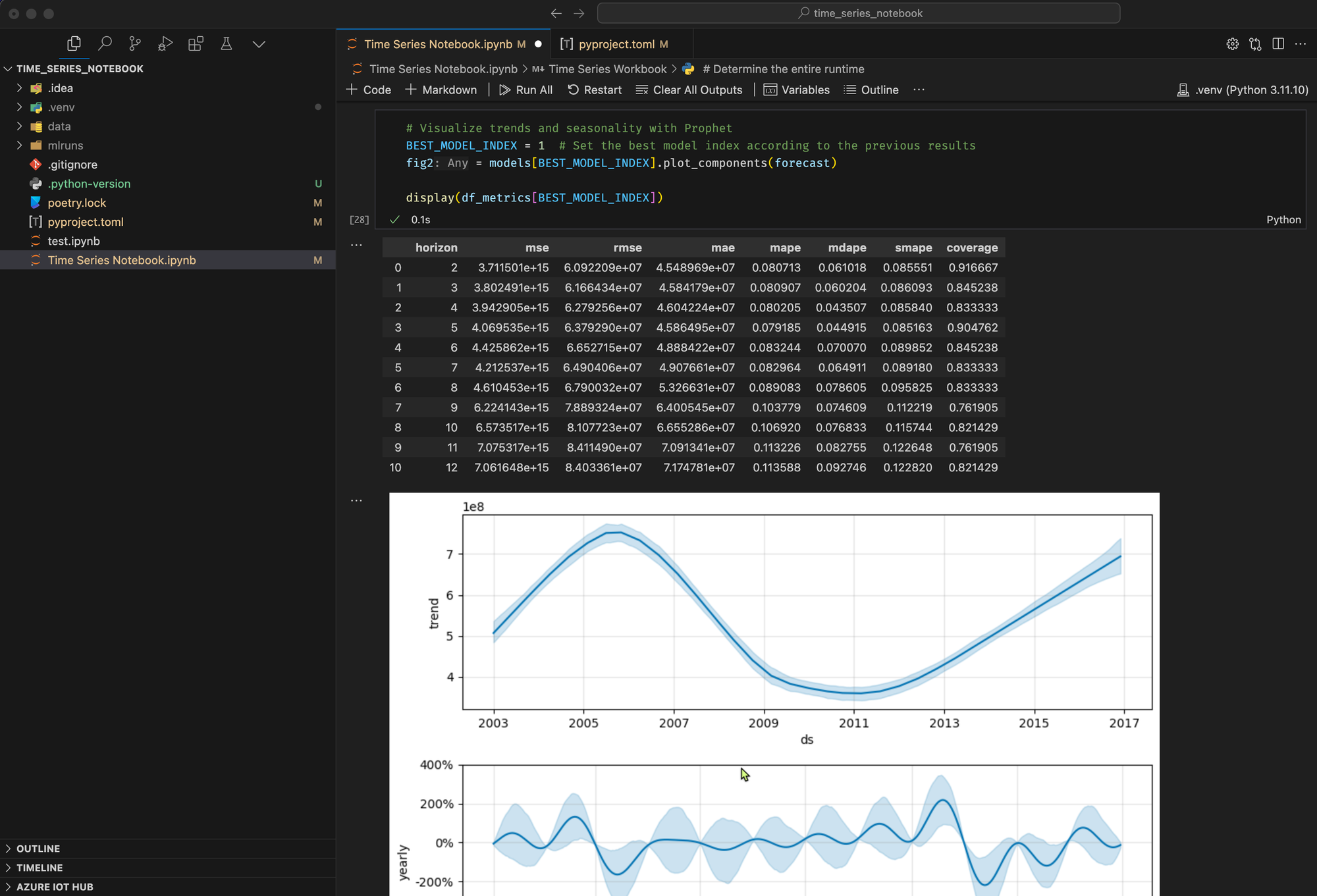
Prophet can also easily visualize the underlying trends and seasonalities. Visualizations of the second model are shown in the results of this code block.
# Visualize trends and seasonality with Prophet
BEST_MODEL_INDEX = 1  # Set the best model index according to the previous results
fig2 = models[BEST_MODEL_INDEX].plot_components(forecast)

display(df_metrics[BEST_MODEL_INDEX])
Score the Model and save Prediction Results
Now score the model, and save the prediction results.
Make Predictions with Predict Transformer
Now, you can load the model and use it to make predictions. Users can operationalize machine learning models with PREDICT, a scalable Microsoft Fabric function that supports batch scoring in any compute engine. Learn more about PREDICT, and how to use it within Microsoft Fabric, at this resource.
We use different Transformers based on whether we run in Fabric or locally.
We also save the predictions in lakehouse or on disk.
# Score the model and save prediction results
test_spark = spark.createDataFrame(data=future, schema=future.columns.to_list())

if is_fabric():
    # Are we running in Fabric/Synapse?
    from synapse.ml.predict import MLFlowTransformer
    spark.conf.set("spark.synapse.ml.predict.enabled", "true")

    model = MLFlowTransformer(
        inputCols=future.columns.values,
        outputCol="prediction",
        modelName=f"{EXPERIMENT_NAME}-prophet",
        modelVersion=BEST_MODEL_INDEX,
    )

    batch_predictions = model.transform(test_spark)
    display(batch_predictions)

    # Code for saving predictions into lakehouse
    batch_predictions.write.format("delta").mode("overwrite").save(
        f"{DATA_FOLDER}/predictions/batch_predictions")

else:
    # Load your data into a pandas DataFrame
    test_pandas = test_spark.toPandas()
    model = models[BEST_MODEL_INDEX]

    # Make predictions
    future['ds'] = pd.to_datetime(future['ds'])  # Ensure the date column is in datetime format
    forecast = model.predict(test_pandas)

    # Display the predictions
    display(forecast[['ds', 'yhat', 'yhat_lower', 'yhat_upper']])

    spark.createDataFrame(forecast).write.format("delta").mode("overwrite").save(
        f"{BASE_FOLDER}/{DATA_FOLDER}/predictions/batch_predictions")
Finally, we can see how much time has elapsed.
# Determine the entire runtime
print(f"Full run cost {int(time.time() - ts)} seconds.")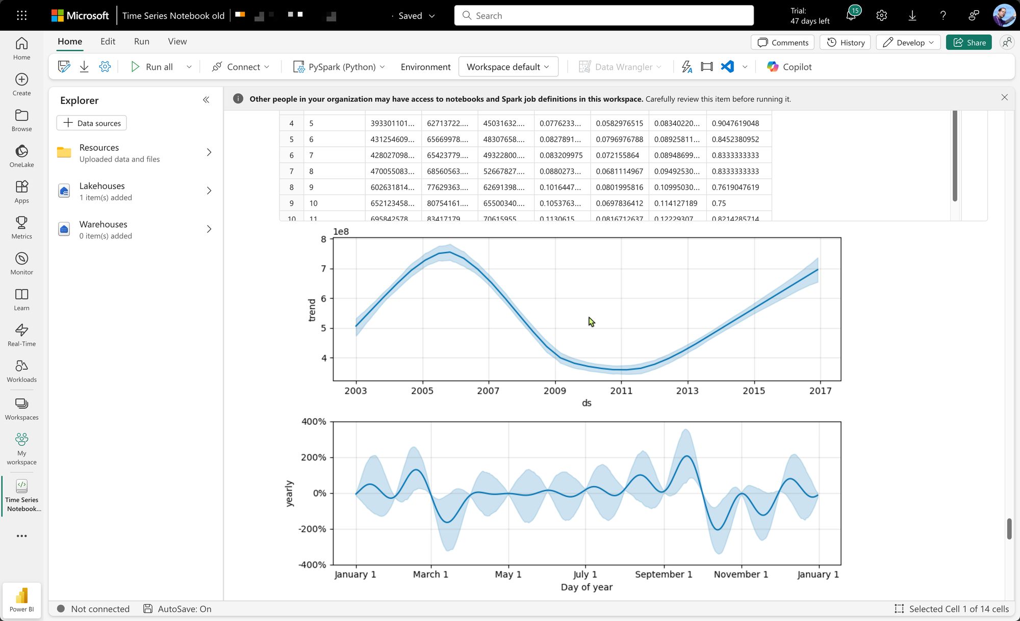
Running Locally
The same workbook will also run locally in any environment that can handle Jupyter notebooks. I'm using VS Code. You will however have to set up a custom, virtual Python environment and install a few requirements which are already present on the Fabric nodes that run your code.
To accomplish this, I have created a Poetry file pyproject.toml:
[tool.poetry]
name = "Time series forecasting"
version = "0.1.0"
description = ""

[tool.poetry.dependencies]
python = "3.11"
seaborn = "^0.13.2"
plotly = "^5.24.1"
prophet = "^1.1.6"
scikit-learn = "^1.5.2"
xgboost = "^2.1.2"
statsmodels = "^0.14.4"
jupyter = "^1.1.1"
pyspark = "^3.5.3"
mlflow = "^2.17.2"
delta-spark = "^3.2.1"

[build-system]
requires = ["poetry-core"]
build-backend = "poetry.core.masonry.api"
To start, create a Python virtual environment with Python 3.11. The libraries used have compatibility issues with higher versions of Python.
In Windows, run the following in your project folder:
py -3.11 -m venv .venv
./.venv/Scripts/activate
On Mac, if you are using pyenv, run this in your project folder:
pyenv local 3.11
pyenv exec python -m venv .venv
./.venv/bin/activate
If you don't have Poetry installed globally, you can add it to the active virtual environment now:
pip install poetryYou can now install the requirements using Poetry:
poetry installAfter a successful installation of all requirements, start VS Code in the current folder:
code .You can now run the notebook from start to end. You will find that all the data will be stored in the ./data subfolder.
